5. Defining Landscape Extents

IMPORTANT

If you’re using Global Mapper, you can follow this process with Tutorial 2.

WE NEED

• The DTM, aerial imagery, and vector data we downloaded in the previous tutorial.
• QGIS. We’re using QGIS V3.12.

Step 1

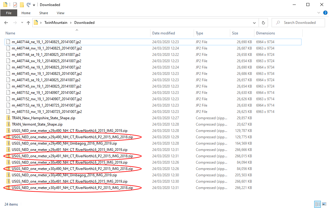
Extract the zip files:

• Extract all the “USGS_NED_*” files into the same folder.
• You can overwrite any files with duplicate names – we don’t need them. Keep the *.img files which contain the data. The rest you can delete if you wish.
• We’ve got some files with duplicate data – it looks like the survey for Twin Mountain was done in both 2018 and 2019 – we’ll delete the duplicate files from 2018 (see below).
• Finally extract the transport (“TRAN_*”) files into separate folders – you don’t want to overwrite files with the same name in those (if you have more than 1)

Step 2

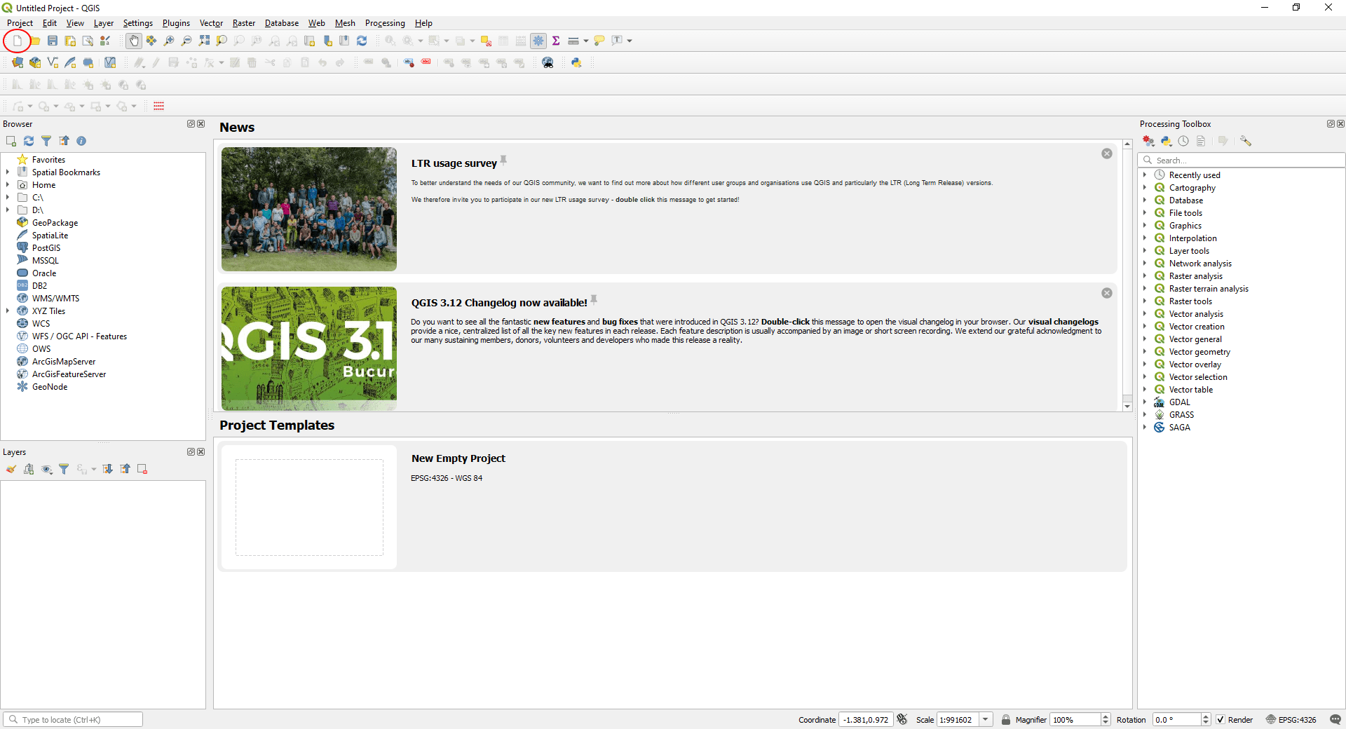
Launch QGIS and create a new project:

• Launch QGIS.
• Click the ‘New Project’ icon under the ‘Project’ menu or on the menu bar.

Step 3

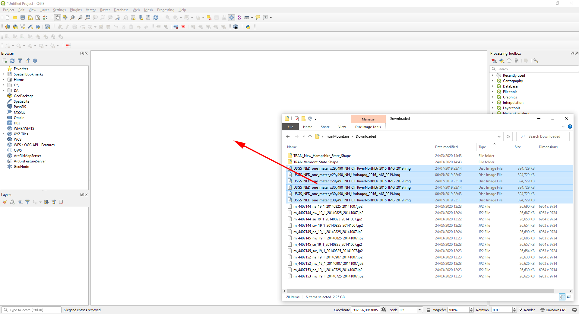
Load DTM files into QGIS:

• QGIS stores data in layers – first loaded appear at the bottom, so we’ll load the DTM data first.
• Launch QGIS from the Programs menu in Windows.
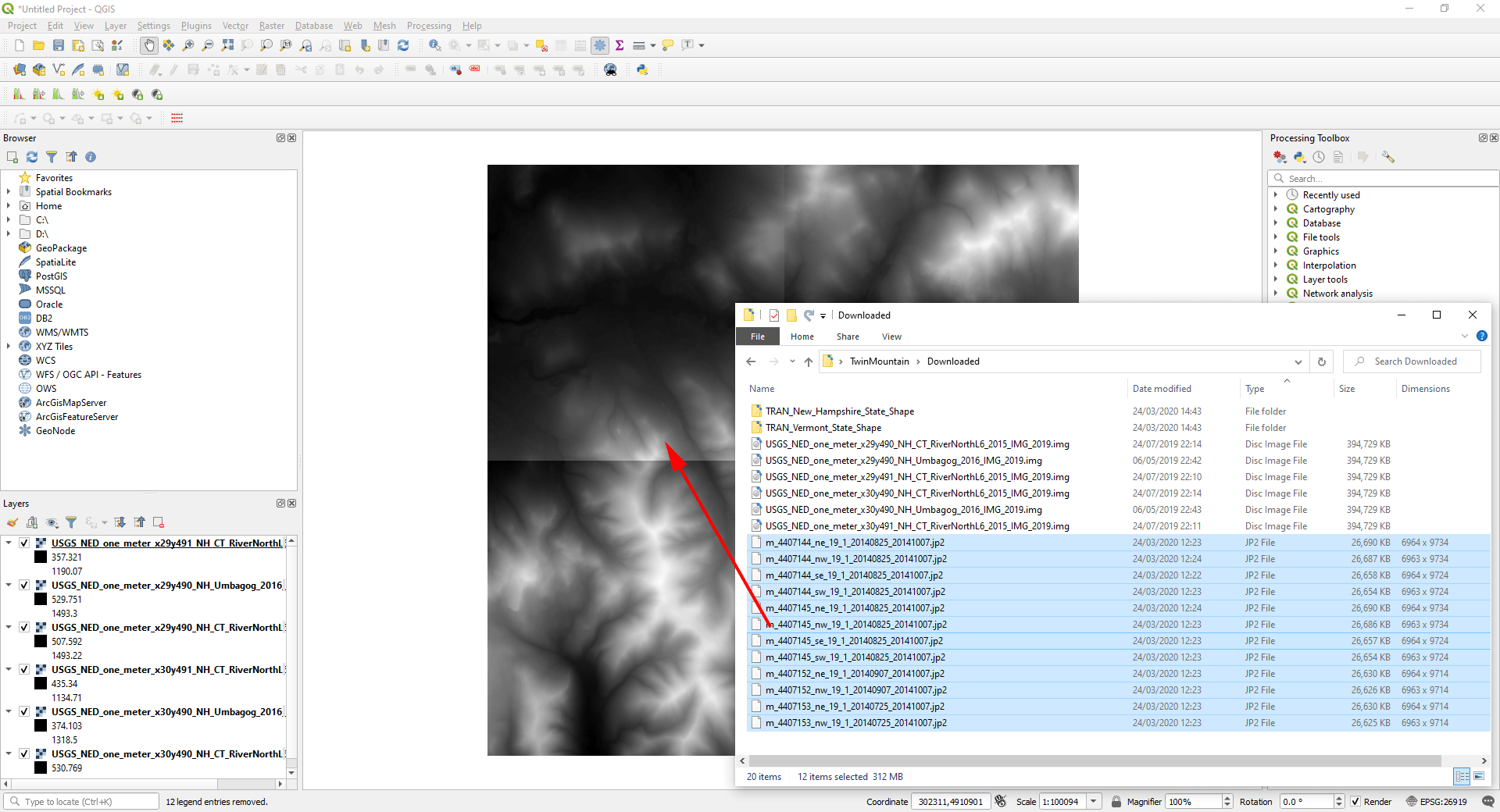
• Select all the .img files in your folder.
• Drag them into the main workspace area in QGIS.

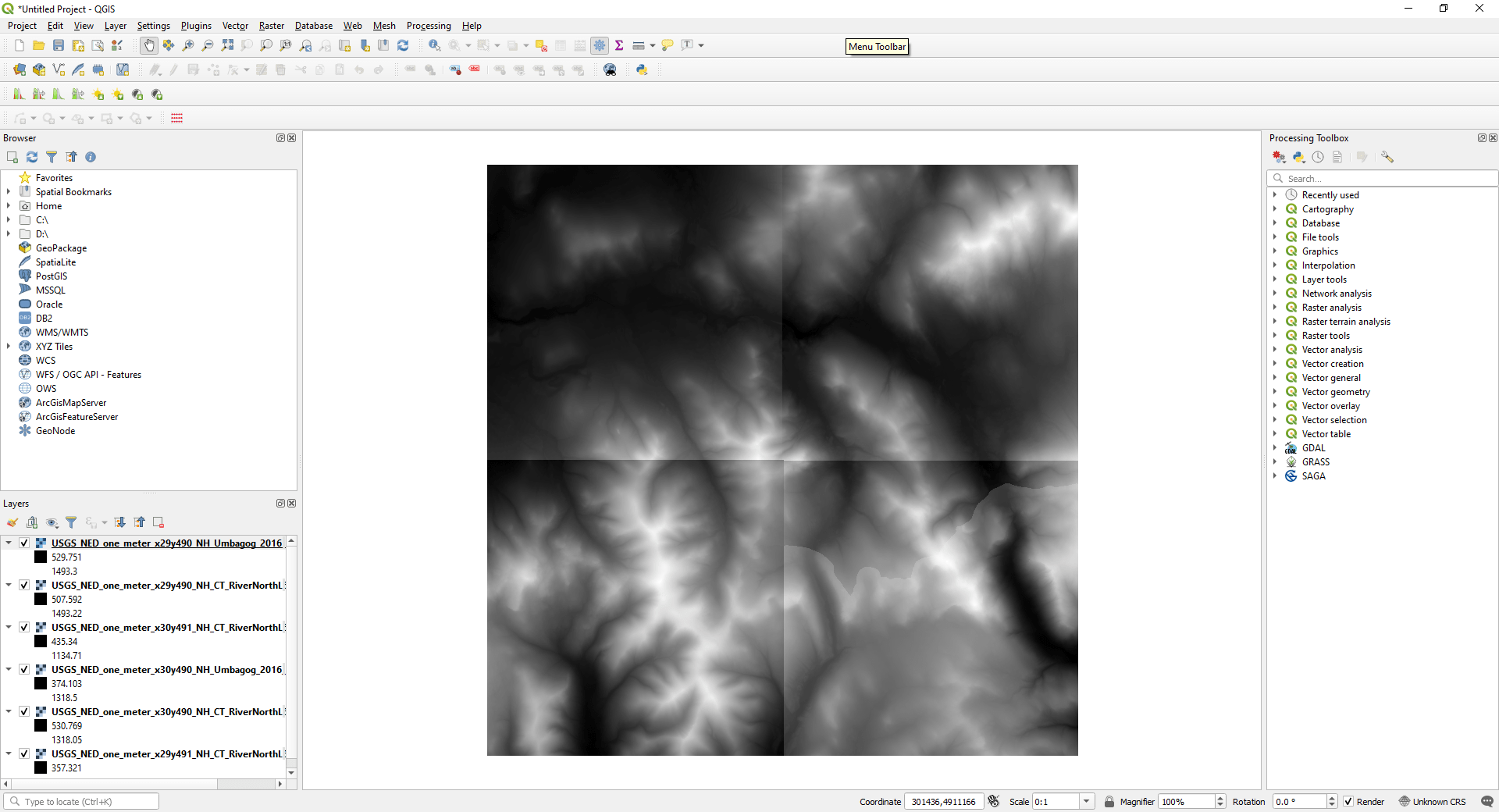
When loaded, the data should look something like this:

Step 4

Check the Projection/Datum have been picked up correctly by QGIS:

[NOTE: The USGS National Elevation Data (NED) is stored in a Cartesian coordinate system known as UTM, and uses the North American Datum defined in 1983 (NAD83). QGIS tries to automatically set the projection and datum for its workspace to those of the first data sets you load, so by loading the NED data first, we should already be working in a local Cartesian coordinate system. (See the status bar in the bottom right of the screenshot below to verify.)]

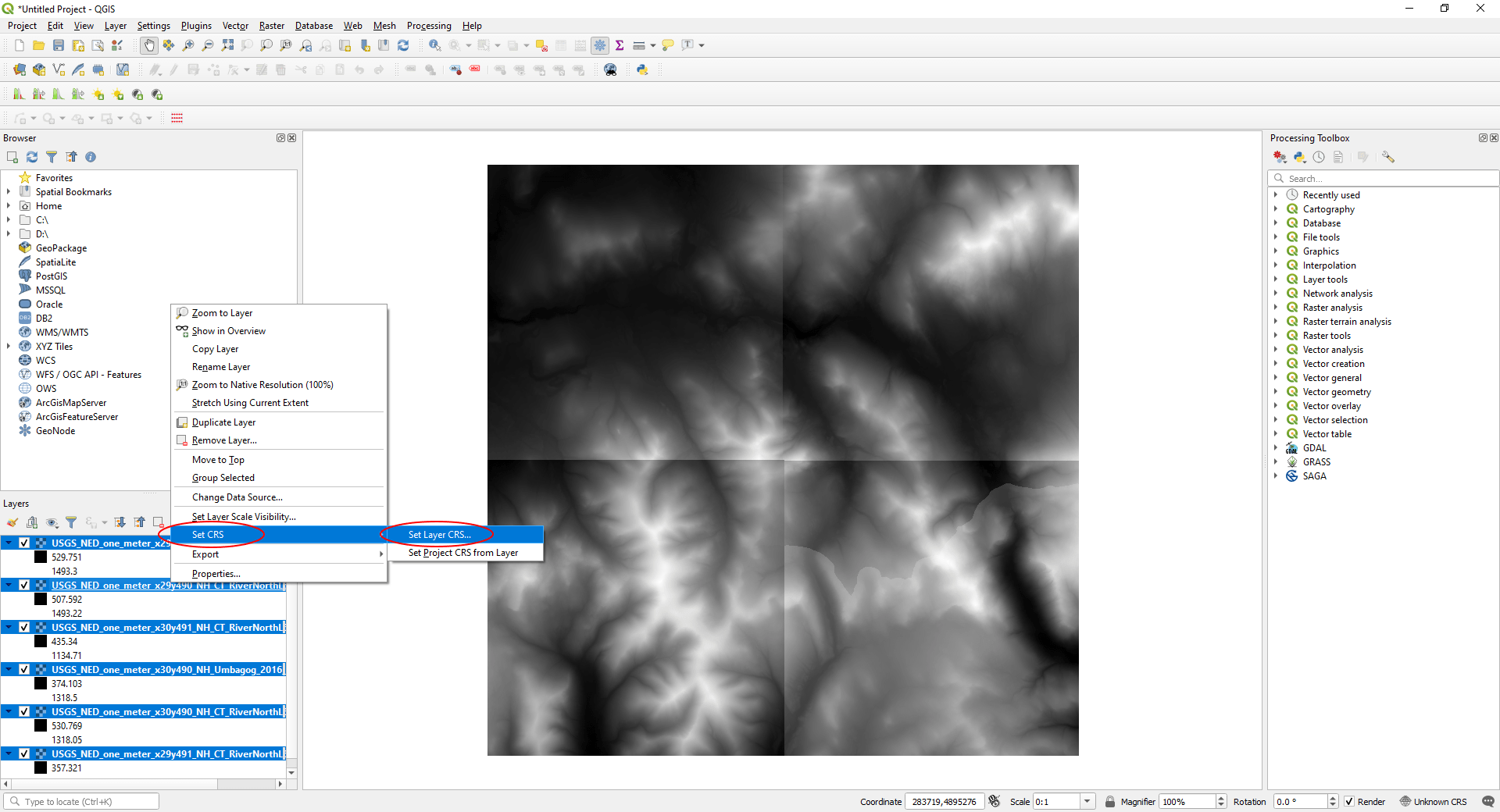
In our case, the Projection/Datum has not been set automatically – we see ‘Unknown CRS’ in the status bar. (CRS stands for “Coordinate Reference System”.)

To fix this:

• Select the DTM layers in the ‘Layers’ tab (hold key and select the first and last layers in the list).
• Then select ‘Set CRS’ > ‘Set Layer CRS…’.

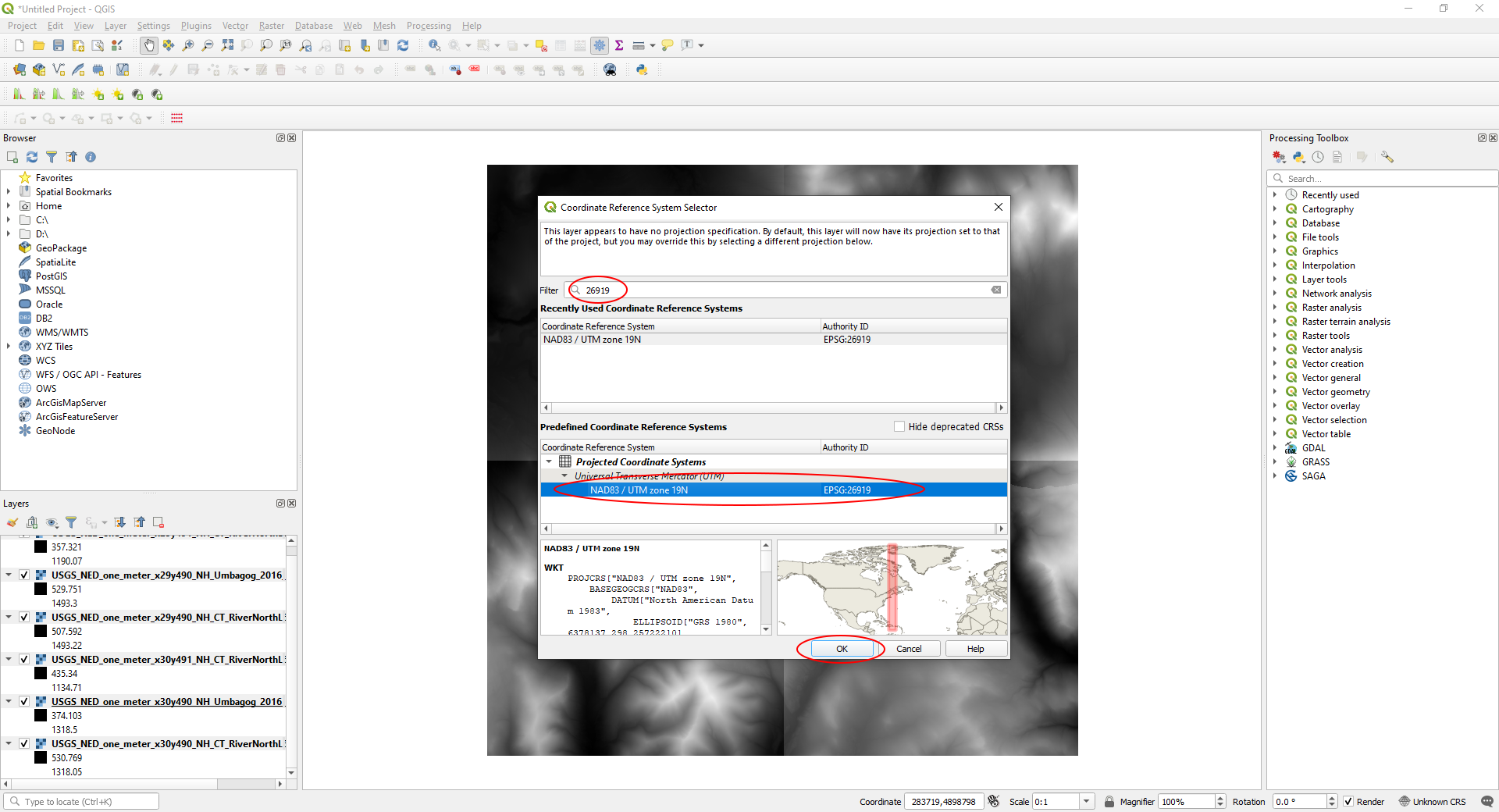
In  the ‘Coordinate Reference System Selector’ window that appears:

• A quick google search tells us ‘EPSG code for UTM Zone 19N NAD83’ is ‘26919’.
• In the ‘Filter’ field, type the EPSG code: 26919 (or as appropriate if you’re using your own data).
• The NAD83/UTM zone 19N is listed in the ‘Predefined Coordinate Reference Systems’ section. Select this.
• Click ‘OK’.

[NOTE: If you’re using your own data, you may need to adjust the projection to a Cartesian system. UTM is a projection that splits the world into local Cartesian ‘Zones’ and is our preferred option. We don’t go into to how to do the re-projection here, but let us know if you’re stuck and we’ll help you out.]

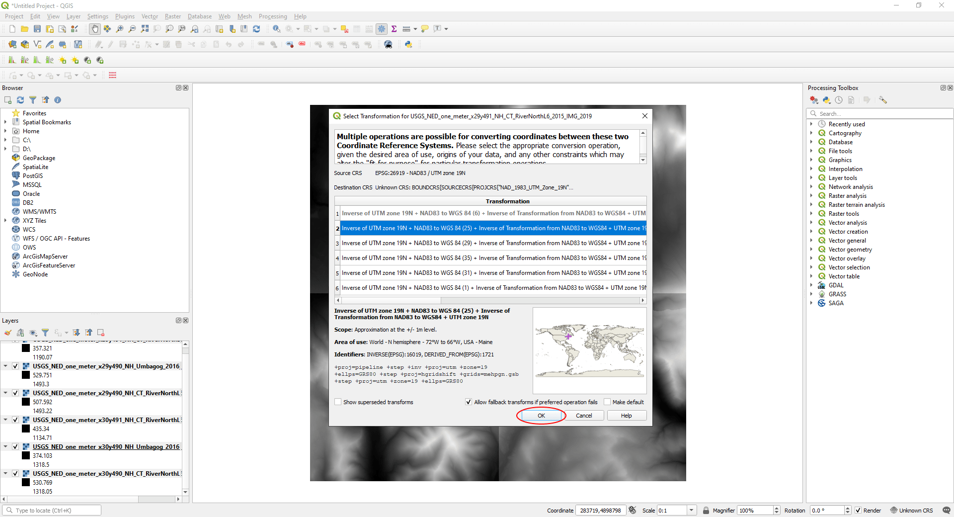
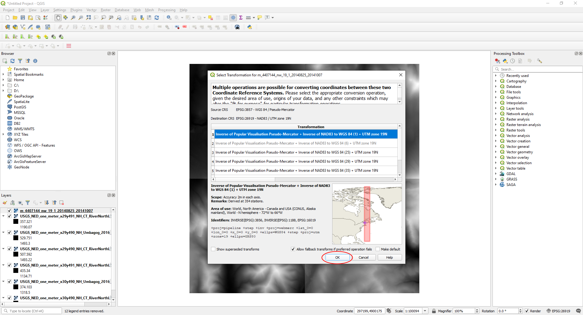
In  the ‘Select Transformation…’ window that appears, leave the default option selected and click ‘OK’.

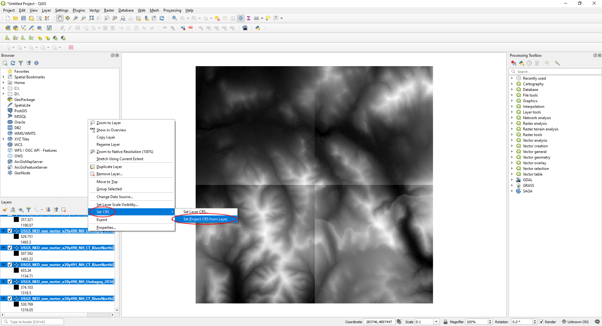
Step 5

Set the ‘Project CRS’ from the DTM data:

• With the DTM layers still selected, again.
• Select ‘Set CRS’ > ‘Set Project CRS from Layer’

Step 6

Load the aerial imagery files into QGIS:

• Select all the .jp2 files in Windows Explorer.
• Drag them into the main QGIS window on top of the loaded DTM files.

In the ‘Select Transforms…’ window that appears, accept the default option by clicking ‘OK’:

Step 7

Load the vector files:

• National Map Viewer listed 2 files for the vectors (New Hampshire and Vermont). Vermont is slightly outside our area of interest, so we don’t need that data.
• When you extracted the “TRAN_*.zip” files, a ‘Shape’ directory should have been created in a sub-folder.
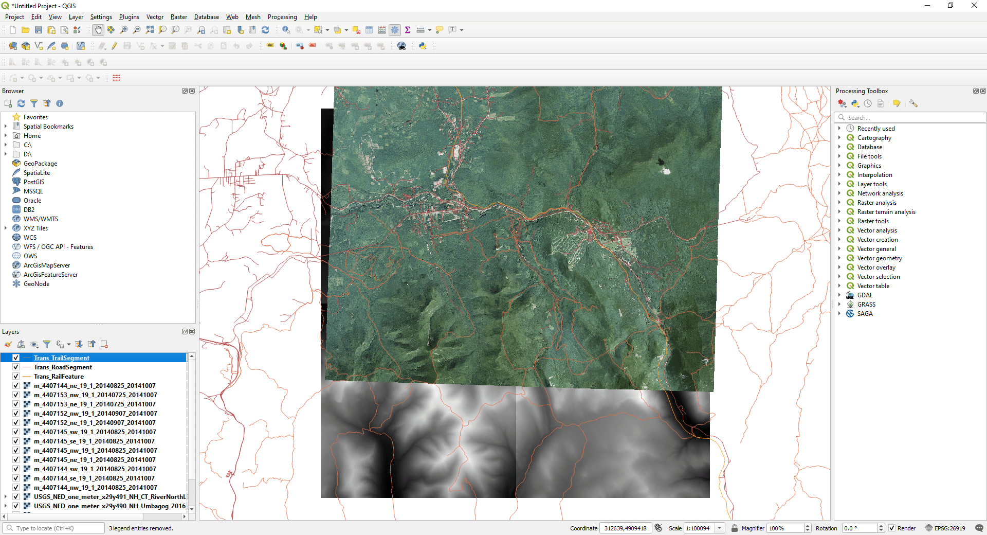
• Select the ‘Trans_RoadSegment.shp’, ‘Trans_RailFeature.shp’, and ‘Trans_TrailSegment.shp’ files and drag them into QGIS:

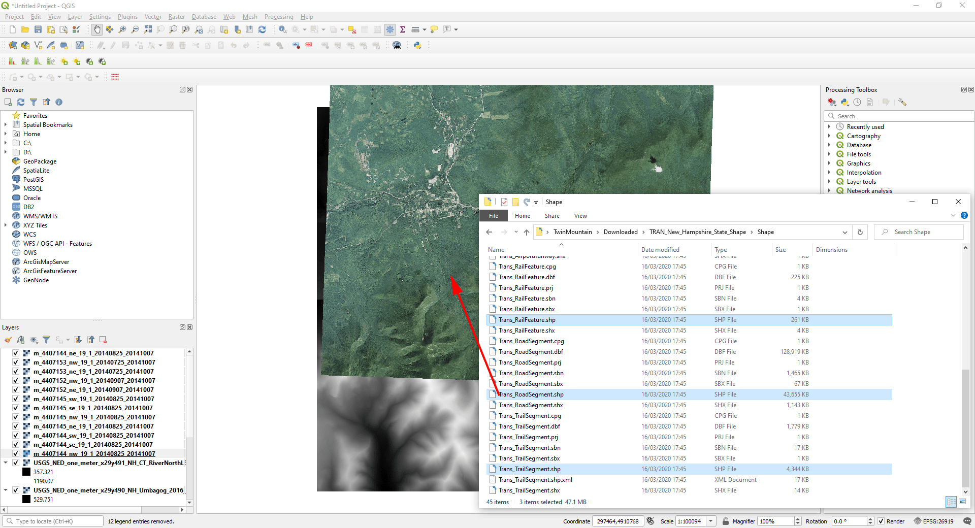
It should look like this:

Step 8

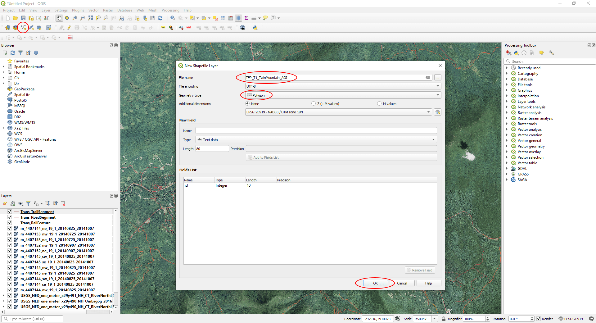
We need to create a box to use as a template to export the data for the area we want to create in UE4:

• The first step is to create a new layer, so click the ‘New ShapeFile Layer…’ icon on the main menu.
• Give it a useful filename.
• Select ‘Polygon’ from the ‘Geometry Type’
• Click ‘OK’.

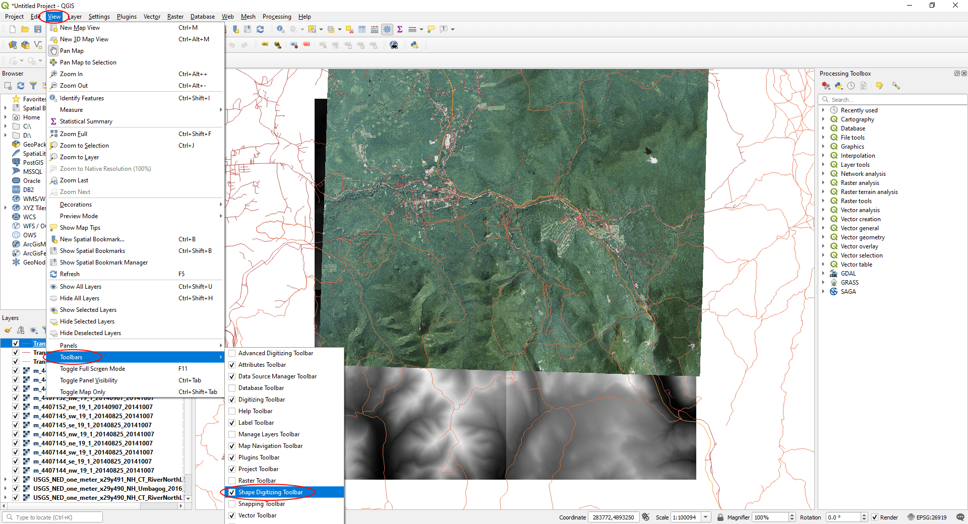
Next, turn on the ‘Shape Digitizer Toolbar’:

• On the main menu, click ‘View’ > ‘Toolbars’
• Make sure the check-box next to ‘Shape Digitizing Toolbar’ is checked.

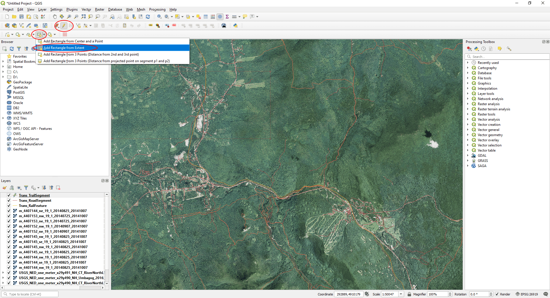
To draw your area:

• Make sure your new layer is selected in the  Layers window.
• Select the ‘Toggle Editing’ icon on the 2nd row of the main toolbar.
• Click the small arrow on the ‘Create Rectangle’ icon in the ‘Shape Digitizer Toolbar’ and from the drop-down list.
• Select  ‘Add Rectangle from Extent’.

[NOTE: You can zoom in and out with the scroll wheel to help you pick your area.]

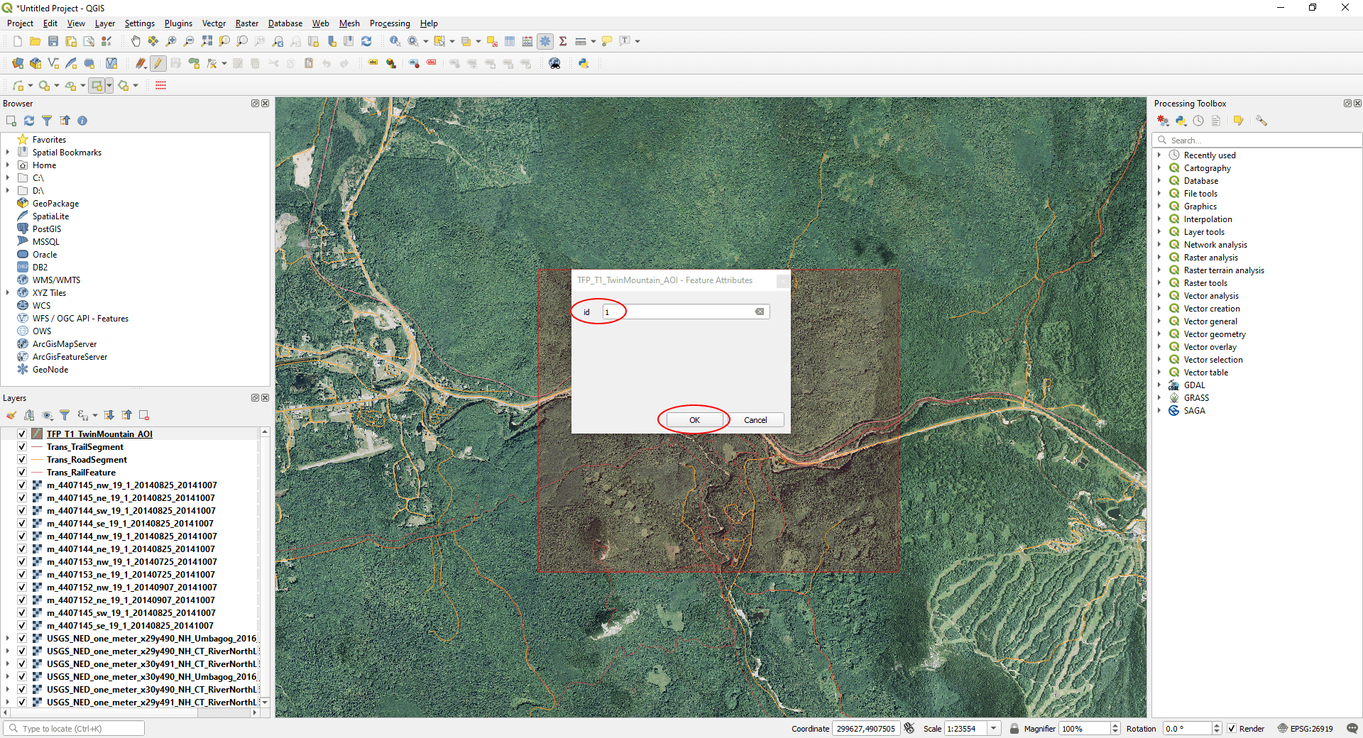
Next:

• <left-click> (and release) where you want the top left corner of your AOI.
• Drag the mouse to where you want the bottom-right corner and <right-click> to stop drawing.
• A ‘Feature Attributes’ window will appear with and ‘ID’ for the shape.
• Integer numbers are required here, so we just enter ‘1’.

[NOTE: You don’t need to export a square area. TerraForm is able to adjust landscape specifications to accommodate rectangular as well as square landscapes.]

Step 9

Now we’re ready to export the data.

Before you do that though, save the Project:

• In QGIS, on the main menu, click ‘Project’ > ‘Save As…’
• Give it a useful name in case you need to refer back to it.